Step 1: Organize Your Data
Ensure your data is organized in a table format with columns and rows. The value you want to look up should be in the first column of the range, and the data you wish to retrieve should be in the same row but can be in any column to the right.
Step 2: Identify the Lookup Value
The lookup value is the data you want to search for in the first column of your table. This could be a name, a number, a date, or any other type of data unique to each row.
Step 3: Determine the Table Array
The table array is the range of cells containing the data you want to search. This includes the column with the lookup value and the columns containing the data you want to retrieve.
Step 4: Specify the Column Index Number
The column index number is the number of the column in the table array from which you want to retrieve data. Count the columns from left to right, starting with the first column as 1.
Step 5: Decide on the Range Lookup
The range lookup is an optional argument that allows you to specify whether you want an exact match (FALSE) or an approximate match (TRUE). If you omit this argument, the default is TRUE.
Example:
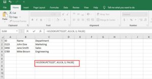
Imagine you have a spreadsheet with employee information. Column A has employee IDs, Column B has names, and Column C has their department. You want to find the department of the employee with ID “E123”.
Here’s how the data might look:
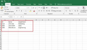
To find John Doe’s department using VLOOKUP, follow these steps:
- Click on the cell where you want the result to appear.
- Enter the VLOOKUP formula:
=VLOOKUP("E123", A1:C3, 3, FALSE) - Press Enter.
Breaking down the formula:
"E123"is the lookup value.A1:C3is the table array.3is the column index number because “Department” is the third column.FALSEspecifies that you want an exact match.
After pressing Enter, Excel will display “Marketing” in the cell where you entered the formula, indicating that John Doe works in the Marketing department.Remember to replace "E123" with the actual cell reference if your lookup value is in a cell, and adjust the table array (A1:C3) to match the range of your actual data.

You can watch Video in here: