In this video we discuss how to subtract a cell, or actually a cell value from a column or row in an excel spreadsheet. We go through a detailed example step by step.
Transcript/notes
Let’s say that you want to subtract a cell value from an entire column, such as in this example excel spreadsheet, where we want to subtract cell D2 from each of the values in the cells in column A, and put the answers in column B.
We start with the first value in cell A2, and we are going to put the answer in cell B2. We start by left clicking on cell B2, so it is highlighted. Next, we type in an equals sign, then we left click on the cell we are subtracting from, in this case cell A2. Now we type in a minus or subtraction sign, then we left click on the cell we are subtracting, in this case cell D2. Then we hit the enter key, and we have our answer of 134.
To make this easy to do for the rest of the answer cells in column B, we are going to adjust the formula we just put into answer cell B2, and I will explain this formula in detail after we have completed the entire process. We again left click on cell B2 so it is highlighted. And we are going to go up into this text box or formula bar here and put the cursor in front of the D and left click. Next, we are going to type in a $, which is shift 4 on the keyboard. From here, we are going to use the arrow key and go over 1 spot to where we are in front of the 2, and we are going to type in another $. And then we will hit the enter key.
You can see that nothing has happened to our answer of 134 in cell B2, which is what we want.
Now, this is where the easy process comes in. To complete the subtraction for the rest of the answer cells in column B, we start again by left clicking on cell B2, so it is highlighted. Next, we are going to move the cursor down to the bottom right hand corner of the cell, and the plus sign will turn black, as you see here. From here, we will left click and hold and drag down to the last cell we need the subtraction from, cell B7. And then we will release the click and hold, and we have completed the subtraction of cell D2 from each of the cells in column A.
Now, going back to the formula in cell B2. By putting in the $ signs before the column letter, D, and the row number, 2, we have given an absolute reference to cell D2, so the rest of the cells will reference the value in that cell when they do the subtraction.
This will also work for rows vs columns, as you see in this example here.
Chapters/Timestamps
0:00 Set up/Intro
0:12 Example subtract cell value from an entire column
0:39 How to adjust formula using “$” (dollar signs)
1:51 Formula explained – absolute reference
2:07 Example for rows


